R-tools

> wiki_username <- "Jouni"
> server <- TRUE
> library(OpasnetUtils)
> library(ggplot2)
> library(reshape2)
> library(plyr)
> ################## Suomentaja
> suomenna <- function(ova) {
+ d <- ova@output
+ if("Trait" %in% colnames(d)) {
+ levels(d$Trait)[levels(d$Trait) == "Cancer"] <- "Syöpä"
+ levels(d$Trait)[levels(d$Trait) == "CHD2"] <- "Sydänkuolema"
+ levels(d$Trait)[levels(d$Trait) == "Stroke"] <- "Aivohalvaus"
+ levels(d$Trait)[levels(d$Trait) == "Child's IQ"] <- "Lapsen ÄO"
+ levels(d$Trait)[levels(d$Trait) == "Tooth defect"] <- "Hammasvaurio"
+ levels(d$Trait)[levels(d$Trait) == "Dental defect"] <- "Hammasvaurio"
+ levels(d$Trait)[levels(d$Trait) == "Vitamin D recommendation"] <- "D-vitamiinin saantisuositus"
+ levels(d$Trait)[levels(d$Trait) == "Dioxin recommendation"] <- "Dioksiinin saantisuositus"
+ }
+ if("Exposure_agent" %in% colnames(ova@output)) {
+ levels(d$Exposure_agent)[levels(d$Exposure_agent) == "Vitamin_D"] <- "D-vitamiini"
+ levels(d$Exposure_agent)[levels(d$Exposure_agent) == "EPA"] <- "EPA"
+ levels(d$Exposure_agent)[levels(d$Exposure_agent) == "DHA"] <- "DHA"
+ levels(d$Exposure_agent)[levels(d$Exposure_agent) == "Omega3"] <- "Omega3"
+ levels(d$Exposure_agent)[levels(d$Exposure_agent) == "PCDDF"] <- "Dioksiini"
+ levels(d$Exposure_agent)[levels(d$Exposure_agent) == "PCB"] <- "PCB"
+ levels(d$Exposure_agent)[levels(d$Exposure_agent) == "TEQ"] <- "TEQ"
+ levels(d$Exposure_agent)[levels(d$Exposure_agent) == "MeHg"] <- "Metyylielohopea"
+ }
+ if("Hedelm" %in% colnames(d)) {
+ levels(d$Hedelm)[levels(d$Hedelm) == FALSE] <- "Ei"
+ levels(d$Hedelm)[levels(d$Hedelm) == TRUE] <- "Kyllä"
+ }
+
+ colnames(d)[colnames(d) == "Age"] <- "Ikäryhmä"
+ colnames(d)[colnames(d) == "Exposure_agent"] <- "Altiste"
+ colnames(d)[colnames(d) == "Trait"] <- "Vaste"
+ colnames(d)[colnames(d) == "Ikä"] <- "Ikä"
+ colnames(d)[colnames(d) == "Silakkamäärä"] <- "Silakkamäärä"
+
+ return(d)
+ }
> ##################### VOI-ANALYYSI
> #objects.latest("Op_en2480", code_name = "Initiate") # Load VOI functions
> VOI <- function(ova, dec) { # Use this simpler total VOI function instead
+ ncpi <- oapply(oapply(ova, cols = dec, FUN = "min"), cols = "Iter", FUN = "mean")
+ ncuu <- oapply(oapply(ova, cols = "Iter", FUN = "mean"), cols = dec, FUN = "min")
+ out <- ncpi - ncuu
+ return(out)
+ }
> ########### HAE RISKITULOKSET JA ALUSTA
> objects.latest("Op_fi3831", code_name = "compute") # Haetaan valmiiksi laskettu indivrisk, pop ja exposure.
> #objects.get("fLcPm8KyLhUuZC0c") # Haetaan tilapäinen versio, jossa on yli 3 g/d saannit typistetty.
> if(exists("server")) BS <- 24 else BS <- 24
> ######################### Pitoisuudet
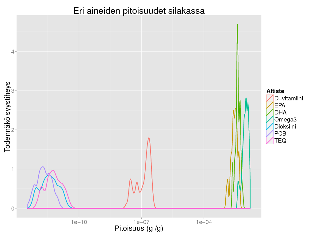
> ggplot(suomenna(concentration), aes(x = Result, colour = Altiste))+geom_density(size = 1)+scale_x_log10() +
+ theme_gray(base_size = BS) + labs(title = "Eri aineiden pitoisuudet silakassa", x = "Pitoisuus (g /g)", y = "Todennäköisyystiheys")
>
> ggplot(suomenna(concentration), aes(y = Result, x = Altiste))+geom_boxplot()+scale_y_log10() +
+ theme_gray(base_size = BS) + labs(title = "Eri aineiden pitoisuudet silakassa", y = "Pitoisuus (g /g)")
> ########################## SILAKANSYÖNTI
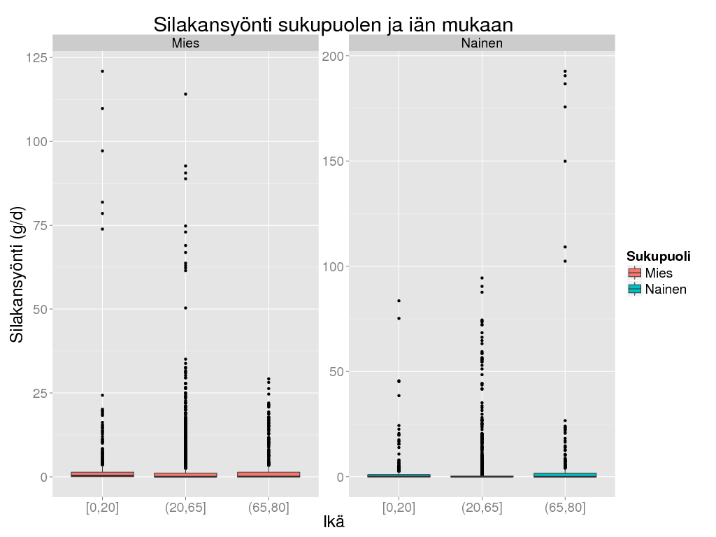
> amount@output$Ikä <- as.numeric(as.character(amount@output$Ikä))
> amount@output$Ikäluokka <- cut(amount@output$Ikä, c(0, 20, 65, 80), include.lowest = TRUE)
> cat("Silakansyönti ikäryhmittäin ja sukupuolittain.\n")

> oprint(summary(amount, marginals = c("Sukupuoli", "Ikäluokka"), fun = c("mean", "sd", "Q0.025", "Q0.975", "length")))

> amo <- suomenna(amount)
> ggplot(subset(amo, Rajoita == "Ei"), aes(x = Result, colour = Ikäluokka)) + stat_ecdf(size = 1) +
+ facet_wrap( ~ Sukupuoli) + scale_x_log10() + theme_gray(base_size = BS) +
+ labs(
+ title = "Silakansyönti sukupuolen ja iän mukaan",
+ colour = "Ikäryhmä",
+ x = "Silakansyönti (g/d)",
+ y = "Kumulatiivinen todennäköisyysjakauma"
+ )
> ggplot(amo, aes(x = cut(Ikä, c(0, 20, 65, 80), include.lowest = TRUE), y = Result, fill = Sukupuoli)) + geom_boxplot() +
+ facet_wrap( ~ Sukupuoli, scale = "free", ncol = 2) + theme_gray(base_size = BS) +
+ labs(
+ title = "Silakansyönti sukupuolen ja iän mukaan",
+ colour = "Ikäryhmä",
+ y = "Silakansyönti (g/d)",
+ x = "Ikä"
+ )
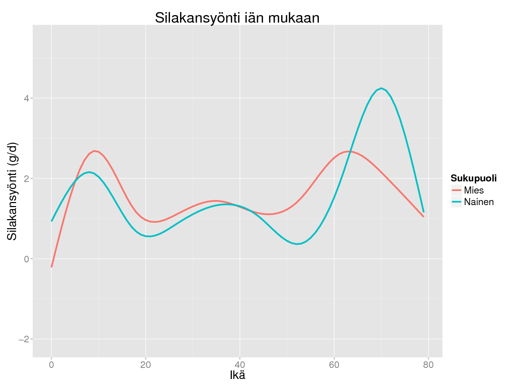
> ggplot(subset(amo, as.integer(as.character(Iter)) <= 1000 & Rajoita == "Ei"), aes(x = Ikä, y = Result, colour = Sukupuoli)) + geom_smooth(size = 1.5) +
+ theme_gray(base_size = BS) + labs(title = "Silakansyönti iän mukaan", y = "Silakansyönti (g/d)")
>
> ######################### ALTISTUKSET
> expo <- suomenna(exposure)
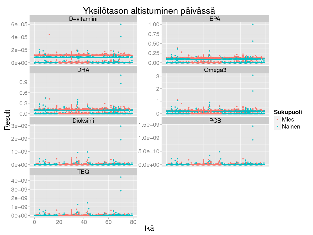
> ggplot(subset(expo, Rajoita == "Ei" & as.integer(as.character(Iter)) <= 1000), aes(x = Ikä, y = Result, colour = Sukupuoli)) + geom_point() +
+ facet_wrap(~ Altiste, scales = "free_y", ncol = 2) + theme_gray(base_size = BS) +
+ labs(title = "Yksilötason altistuminen päivässä")
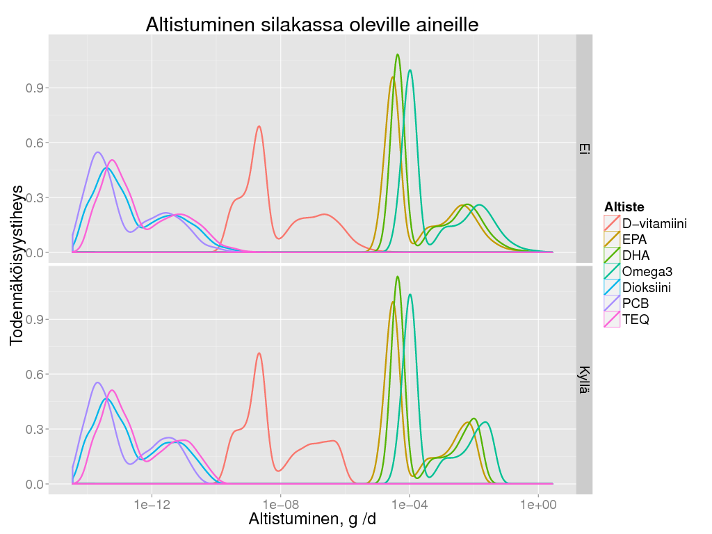
> ggplot(subset(expo, Tausta == "Ei"), aes(x = Result, colour = Altiste)) + geom_density(size = 1) + scale_x_log10() + facet_grid(Rajoita ~ .) +
+ labs(
+ title = "Altistuminen silakassa oleville aineille",
+ y = "Todennäköisyystiheys",
+ x = "Altistuminen, g /d") +
+ theme_gray(base_size = BS)
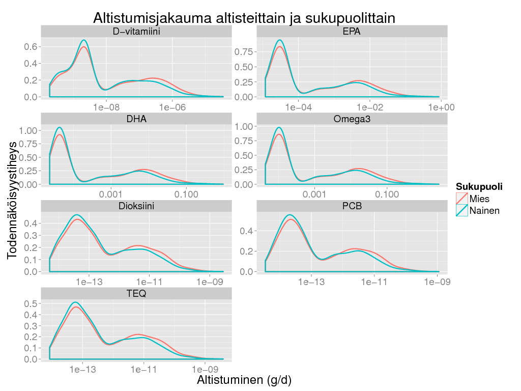
> ggplot(subset(expo, Tausta == "Ei" & Rajoita == "Ei"), aes(x = Result, colour = Sukupuoli)) + geom_density(size = 1) +
+ facet_wrap( ~ Altiste, scale = "free", ncol = 2) + scale_x_log10() + theme_gray(base_size = BS) +
+ labs(
+ title = "Altistumisjakauma altisteittain ja sukupuolittain",
+ y = "Todennäköisyystiheys",
+ x = "Altistuminen (g/d)")
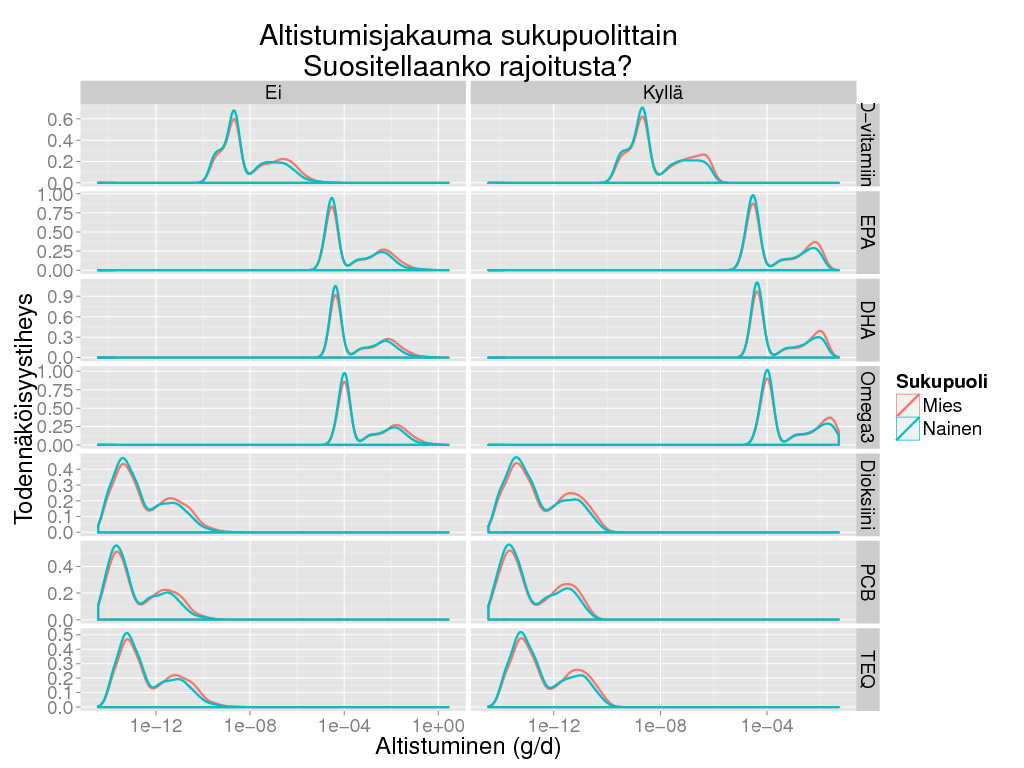
> ggplot(subset(expo, Tausta == "Ei"), aes(x = Result, colour = Sukupuoli)) + geom_density(size = 1) +
+ facet_grid(Altiste ~ Rajoita , scale = "free") + scale_x_log10() + theme_gray(base_size = BS) +
+ labs(title = "Altistumisjakauma sukupuolittain\nSuositellaanko rajoitusta?",
+ x = "Altistuminen (g/d)",
+ y = "Todennäköisyystiheys")
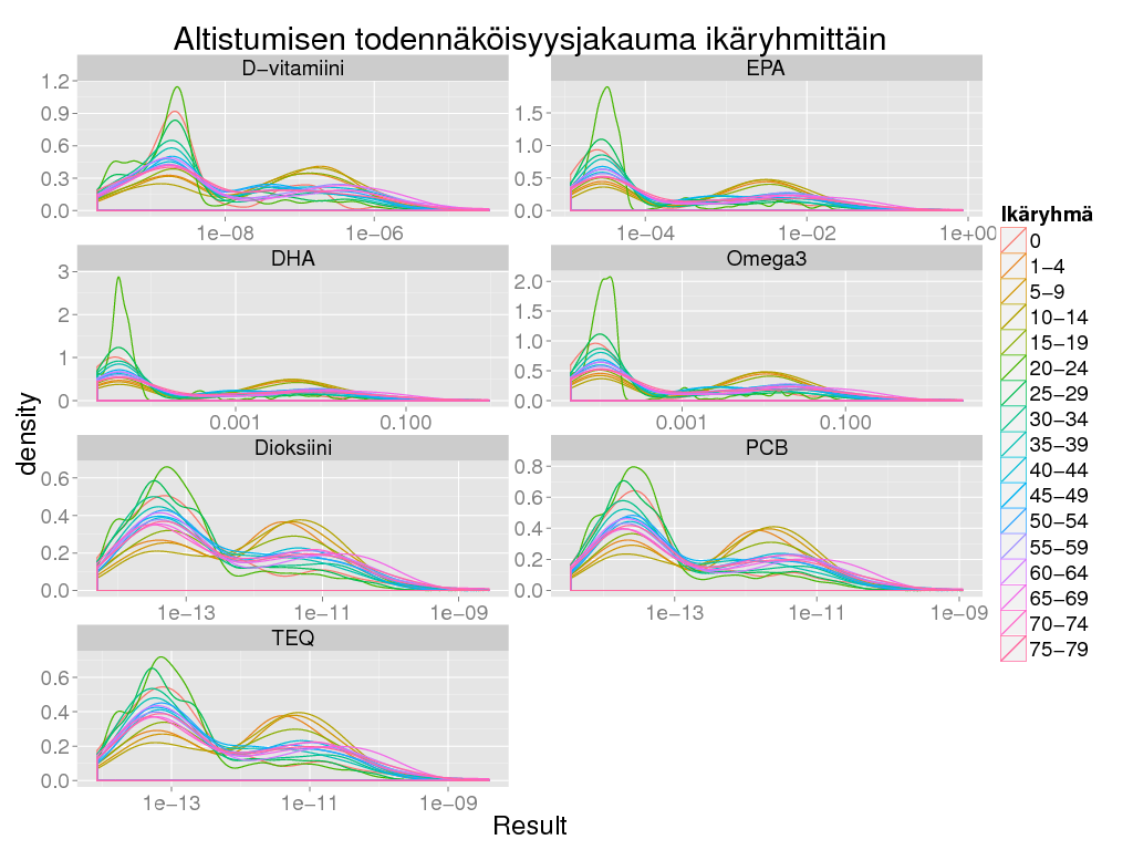
> ggplot(subset(expo, Rajoita == "Ei" & Tausta == "Ei"), aes(x = Result, colour = Ikäryhmä)) + geom_density() +
+ facet_wrap( ~ Altiste, scale = "free", ncol = 2) + scale_x_log10() + theme_gray(base_size = BS) +
+ labs(title = "Altistumisen todennäköisyysjakauma ikäryhmittäin")
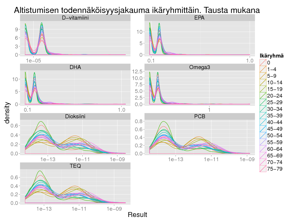
> ggplot(subset(expo, Rajoita == "Ei" & Tausta == "Kyllä"), aes(x = Result, colour = Ikäryhmä)) + geom_density() +
+ facet_wrap( ~ Altiste, scale = "free", ncol = 2) + scale_x_log10() + theme_gray(base_size = BS) +
+ labs(title = "Altistumisen todennäköisyysjakauma ikäryhmittäin. Tausta mukana")
> ################################ VÄESTÖTIETO JA PAINOKERTOIMET
> dweight <- Ovariable("dweight", ddata = "Op_fi3831.laatupainotetut_elinvuodet_vaikutuksille")
> dweight@data$Response_metric <- NULL
> daly <- unkeep(indivrisk * dweight, sources = TRUE, prevresults = TRUE)
> daly@output <- subset(daly@output, Trait != "Dioxin recommendation")
> # pophed is the population size for each Hedelm * Age subgroup. This can be summed over either Hedelm or Age.
> # pophed is for a single sex, so it should be multiplied with an ovariable with index Sex to get values for the whole population.
> pophed <- pop / 2 * Ovariable(
+ output = data.frame(unique(daly@output[c("Hedelm", "Age")]), Result = 1),
+ marginal = c(TRUE, TRUE, FALSE)
+ )
> ############################# RYHMÄKOHTAISET DALYT
> # daly: all DALYs (contains exposure and non-exposure scenarios)
> ## dalyp: DALYs on population level, i.e. daly multiplied by subgroup sizes.
> ## dalyi: individual DALYs summed over Traits
> dalyp <- daly * pophed
> cat("Silakansyönnin DALYt vasteen, sukupuolen ja politiikkojen mukaan.\n")

> # Jokin vika eli ei käytetä J-unitseja
> #library(scales)
> #junit_trans = function() trans_new("junit", function(x) x^(1/3), function(x) x^3)
> #ggplot(data.frame(Result = -50:50), aes(x = Result)) + geom_density() + coord_trans(x = "junit") + labs(title = "Kuva 7. Todennäköisyyden tiheysjakauma ikäryhmittäin")
> #Error in if (zero_range(range)) { : missing value where TRUE/FALSE needed
> ############################# DALYT IKÄRYHMITTÄIN
> d1 <- subset(suomenna(dalyp), Rajoita == "Ei")
> Nd <- as.data.frame(as.table(tapply(d1$Iter, d1[c("Rajoita", "Vaste", "Sukupuoli", "Hedelm", "Tausta", "Ikäryhmä")], FUN = length)))
> Nd <- Nd[!is.na(Nd$Freq) , ]
> d1 <- merge(d1, Nd)
> test1 <- !d1$Ikäryhmä %in% c("50-54", "55-59", "60-64", "65-69", "70-74", "75-79")
> # Tämä varmistaa, että pylväät eivät pilkkoudu kirjaviksi
> d1 <- d1[order(d1$Vaste) , ]
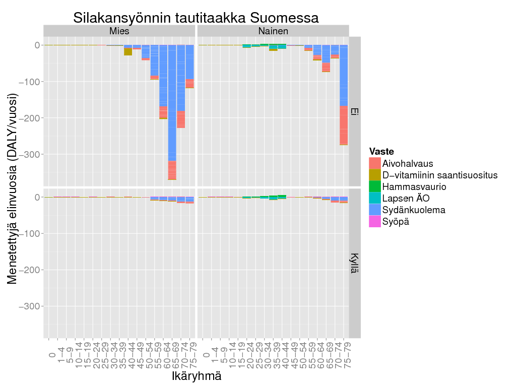
> ggplot() +
+ geom_bar(data = subset(d1, Result > 0), aes(x = Ikäryhmä, y = Result/Freq, fill = Vaste), stat = "identity") +
+ geom_bar(data = subset(d1, Result <= 0), aes(x = Ikäryhmä, y = Result/Freq, fill = Vaste), stat = "identity") +
+ facet_grid(Tausta ~ Sukupuoli) + theme_gray(base_size = BS) +
+ labs(title = "Silakansyönnin tautitaakka Suomessa",
+ y = "Menetettyjä elinvuosia (DALY/vuosi)") + theme(axis.text.x = element_text(angle = 90))
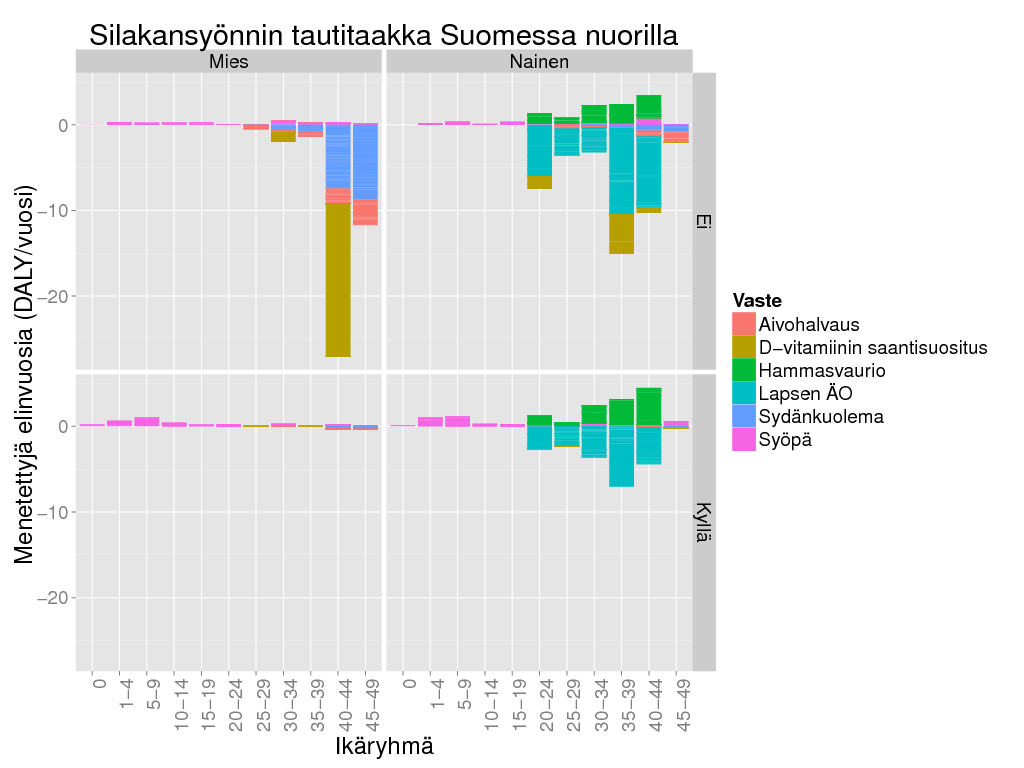
> ggplot() +
+ geom_bar(data = subset(d1, test1 & Result > 0), aes(x=Ikäryhmä, y = Result/Freq, fill = Vaste), stat = "identity") +
+ geom_bar(data = subset(d1, test1 & Result <= 0), aes(x=Ikäryhmä, y = Result/Freq, fill = Vaste), stat = "identity") +
+ facet_grid(Tausta ~ Sukupuoli) + theme_gray(base_size = BS) + theme(axis.text.x = element_text(angle = 90, hjust = 1)) +
+ labs(title = "Silakansyönnin tautitaakka Suomessa nuorilla",
+ y = "Menetettyjä elinvuosia (DALY/vuosi)") + theme(axis.text.x = element_text(angle = 90))
> ############################## VÄESTÖTASON MUUTOKSET RAJOITUSPOLITIIKAN TAKIA
> d2 <- dalyp * Ovariable(output = data.frame(Rajoita = c("Kyllä", "Ei"), Result = c(1, -1)), marginal = c(TRUE, FALSE))
> d2 <- suomenna(oapply(d2, INDEX = c("Trait", "Sukupuoli", "Iter", "Tausta", "Age"), FUN = sum))
> Nd <- as.data.frame(as.table(tapply(d2$Iter, d2[c("Vaste", "Sukupuoli", "Tausta", "Ikäryhmä")], FUN = length)))
> Nd <- Nd[!is.na(Nd$Freq) , ]
> d2 <- merge(d2, Nd)
> d2 <- d2[order(d2$Vaste, d2$Ikäryhmä, d2$Sukupuoli) , ]
> test2 <- !d2$Ikäryhmä %in% c("50-54", "55-59", "60-64", "65-69", "70-74", "75-79", "80-84", "85-89", "90-94", "95-")
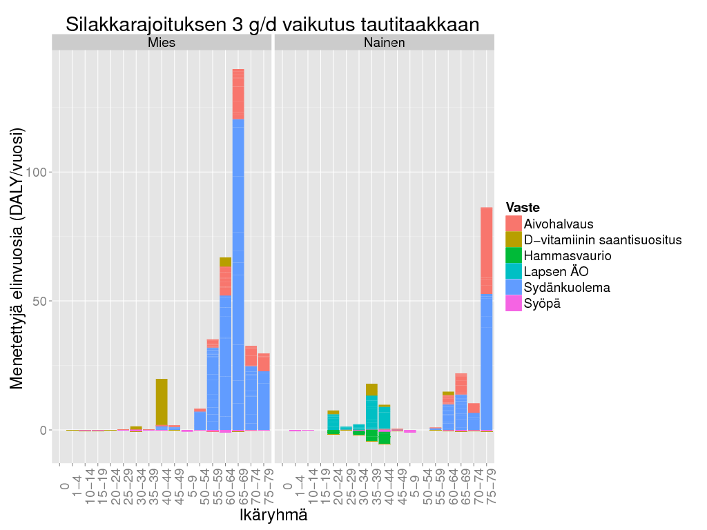
> ggplot() +
+ geom_bar(data = subset(d2, Result > 0), aes(x = Ikäryhmä, y = Result/Freq, fill = Vaste), stat = "identity") +
+ geom_bar(data = subset(d2, Result <= 0), aes(x = Ikäryhmä, y = Result/Freq, fill = Vaste), stat = "identity") +
+ facet_grid(. ~ Sukupuoli) + theme_gray(base_size = BS) +
+ labs(title = "Silakkarajoituksen 3 g/d vaikutus tautitaakkaan",
+ y = "Menetettyjä elinvuosia (DALY/vuosi)") + theme(axis.text.x = element_text(angle = 90))
> ggplot() +
+ geom_bar(data = subset(d2, test2 & Result > 0), aes(x=Ikäryhmä, y = Result/Freq, fill = Vaste), stat = "identity") +
+ geom_bar(data = subset(d2, test2 & Result <= 0), aes(x=Ikäryhmä, y = Result/Freq, fill = Vaste), stat = "identity") +
+ facet_grid(Tausta ~ Sukupuoli) + theme_gray(base_size = BS) + theme(axis.text.x = element_text(angle = 90, hjust = 1)) +
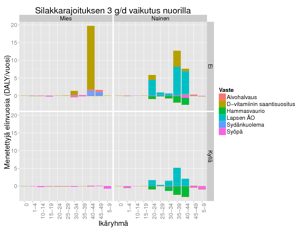
+ labs(title = "Silakkarajoituksen 3 g/d vaikutus nuorilla",
+ y = "Menetettyjä elinvuosia (DALY/vuosi)") + theme(axis.text.x = element_text(angle = 90))
> ######################### YKSILÖRISKIT ERI VASTEILLE
> riski <- subset(suomenna(indivrisk), Tausta == "Ei" & Rajoita == "Ei" & Iter <= 1000)
> ggplot(riski, aes(x = Ikä, y = Result)) +
+ geom_point() + geom_smooth() +
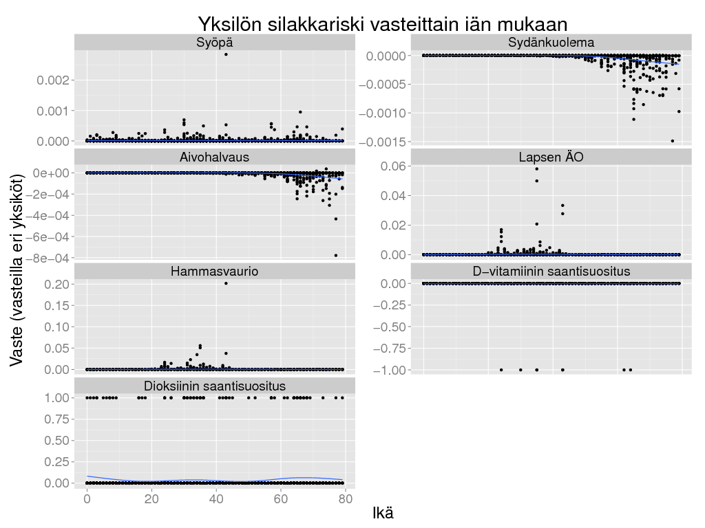
+ facet_wrap(~ Vaste, scale = "free_y", ncol = 2)+ theme_gray(base_size = BS) +
+ labs(title = "Yksilön silakkariski vasteittain iän mukaan",
+ y = "Vaste (vasteilla eri yksiköt)")
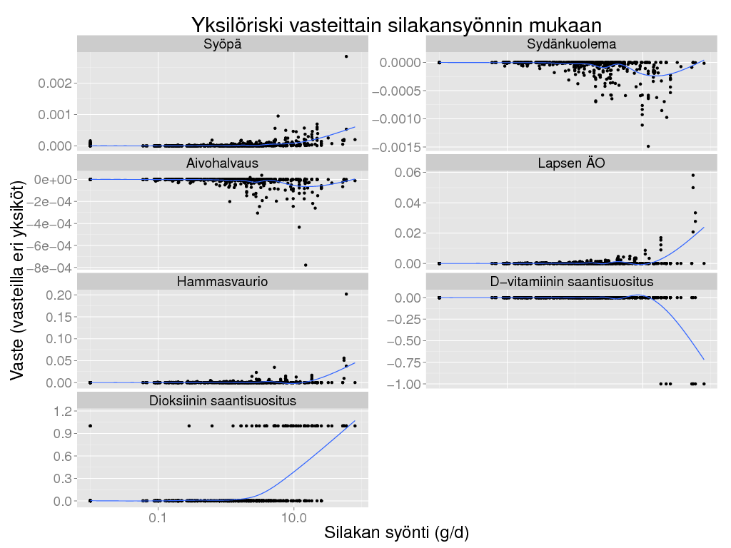
> ggplot(riski, aes(x = Silakkamäärä, y = Result)) + geom_point() + geom_smooth() + theme_gray(base_size = BS) + scale_x_log10() +
+ facet_wrap(~ Vaste, ncol = 2, scale = "free_y") +
+ labs(title = "Yksilöriski vasteittain silakansyönnin mukaan",
+ x = "Silakan syönti (g/d)",
+ y = "Vaste (vasteilla eri yksiköt)")
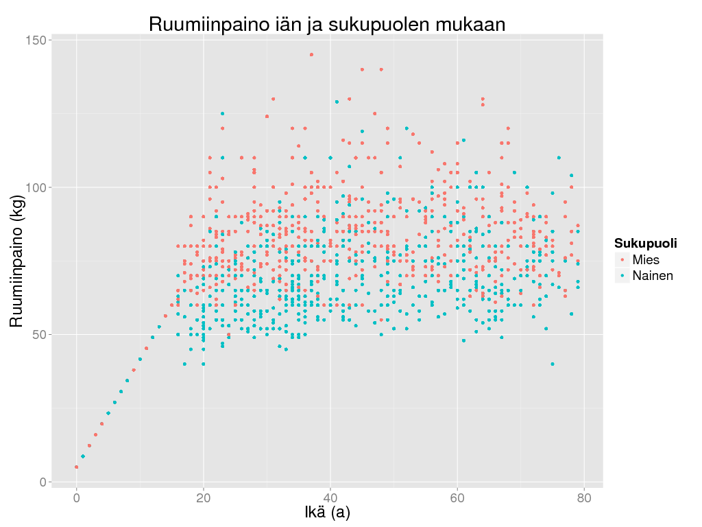
> ggplot(riski, aes(x = Ikä, y = Paino, colour = Sukupuoli)) +
+ geom_point() + theme_gray(base_size = BS) +
+ labs(title = "Ruumiinpaino iän ja sukupuolen mukaan",
+ x = "Ikä (a)",
+ y = "Ruumiinpaino (kg)"
+ )
> ######################## YKSILÖLLISET DALYT
> dalyi <- oapply(daly, INDEX = c("Sukupuoli", "Iter", "Rajoita", "Tausta", "Age"), FUN = sum, use_plyr = TRUE)
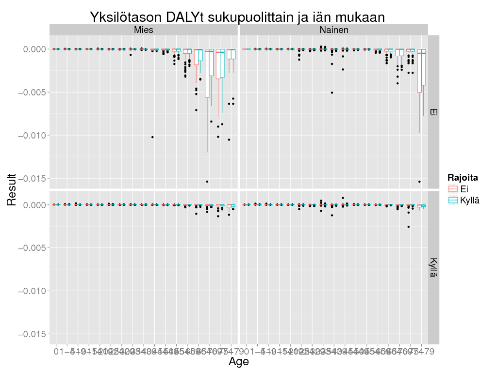
> ggplot(dalyi@output, aes(x = Age, y = Result, colour = Rajoita)) + geom_boxplot() + theme_gray(base_size = BS) +
+ facet_grid(Tausta ~ Sukupuoli) +
+ labs(title = "Yksilötason DALYt sukupuolittain ja iän mukaan")
> ggplot(dalyi@output, aes(x = Age, y = Result, colour = Rajoita)) + geom_boxplot() + theme_gray(base_size = BS) +
+ facet_grid(Tausta ~ Sukupuoli) + coord_cartesian(ylim = c(-0.005, 0.001)) +
+ labs(title = "Yksilötason DALYt sukupuolittain ja iän mukaan", y = "DALY/a (Rajattu alue)")
> # Look at individual risks and probability that the herring eating recommendation is correct.
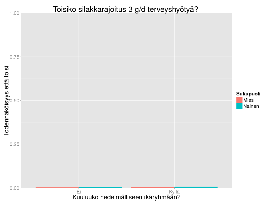
> dalyir <- oapply(daly, cols = c("Trait"), FUN = "sum")
> dalyir3 <- dalyir * Ovariable(output = data.frame(Rajoita = c("Kyllä", "Ei"), Result = c(1, -1)), marginal = c(TRUE, FALSE))
> dalyir3 <- oapply(dalyir3, INDEX = c("Sukupuoli", "Iter", "Hedelm"), FUN = sum)
> dalyir3 <- oapply(dalyir3, INDEX = c("Sukupuoli", "Hedelm"), FUN = function(x) sum(x <= -0.00003) / length(x))
> # Terveysvaikutuksen rajana 1 terve päivä elinaikana (1/365/80) enemmän.
> ggplot(suomenna(dalyir3), aes(x = Hedelm, weight = Result, fill = Sukupuoli)) +
+ geom_bar(position = "dodge") + theme_gray(base_size = BS) +
+ coord_cartesian(ylim = c(0,1)) +
+ labs(
+ title = "Toisiko silakkarajoitus 3 g/d terveyshyötyä?",
+ y = "Todennäköisyys että toisi",
+ x = "Kuuluuko hedelmälliseen ikäryhmään?"
+ )
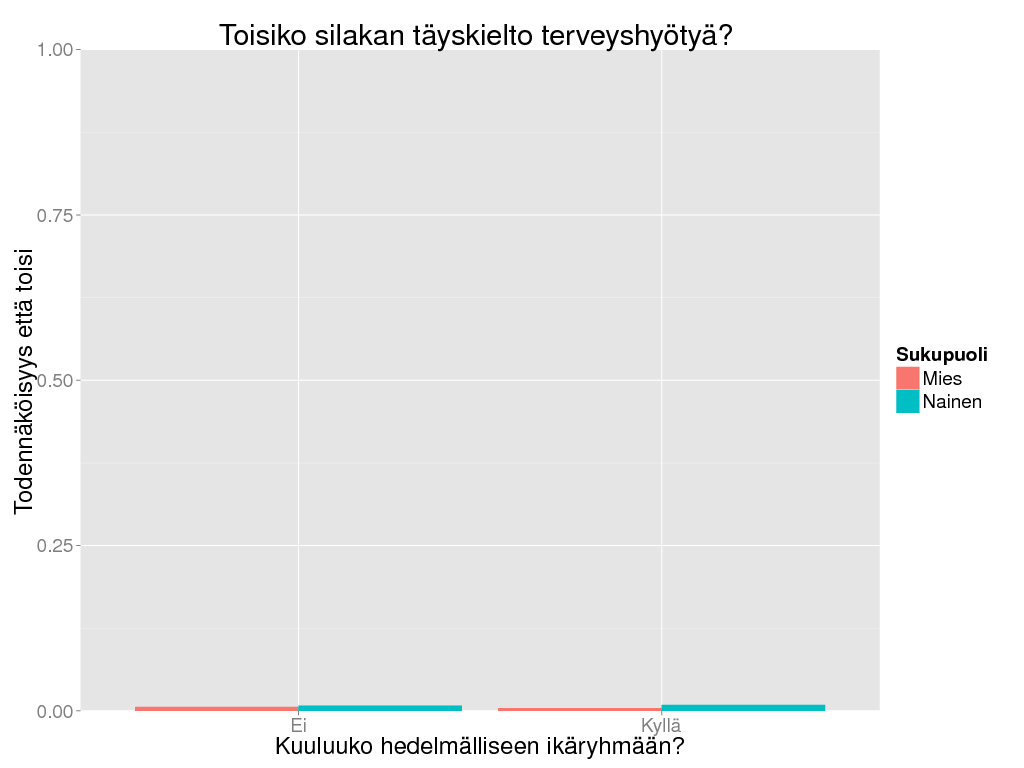
> ## Look at recommendation of total herring ban.
> dalyir0 <- dalyir * Ovariable(output = data.frame(Rajoita = c("Kyllä", "Ei"), Result = c(0, -1)), marginal = c(TRUE, FALSE))
> dalyir0 <- oapply(dalyir0, INDEX = c("Sukupuoli", "Iter", "Hedelm"), FUN = sum)
> dalyir0 <- oapply(dalyir0, INDEX = c("Sukupuoli", "Hedelm"), FUN = function(x) sum(x <= -0.00003) / length(x))
> ggplot(suomenna(dalyir0), aes(x = Hedelm, weight = Result, fill = Sukupuoli)) +
+ geom_bar(position = "dodge") + theme_gray(base_size = BS) +
+ coord_cartesian(ylim = c(0,1)) +
+ labs(
+ title = "Toisiko silakan täyskielto terveyshyötyä?",
+ y = "Todennäköisyys että toisi",
+ x = "Kuuluuko hedelmälliseen ikäryhmään?"
+ )
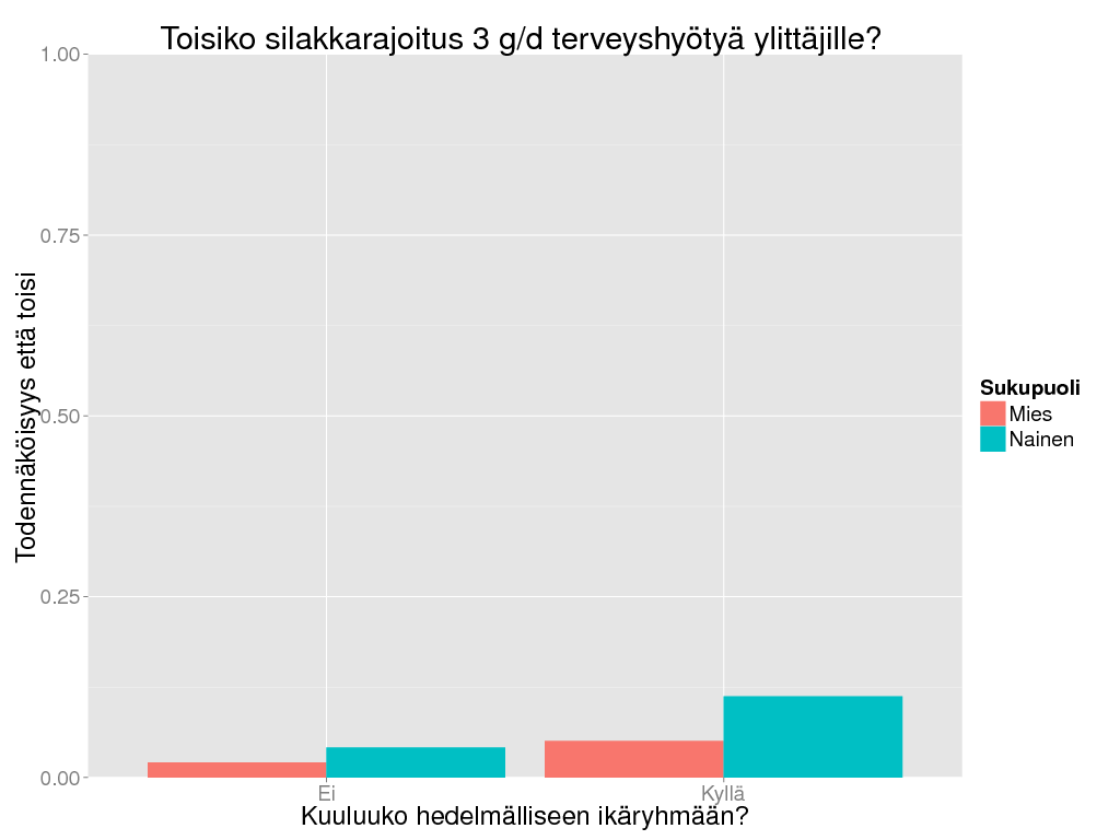
> # Look at individual risks and probability that the herring eating recommendation is correct.
> # WITHIN THE POPULATION THAT ATE >= 3 g/d
> daly3n <- amount
> daly3n@output <- subset(daly3n@output, Rajoita == "Ei")
> daly3n <- dalyir3 / oapply(daly3n, INDEX = c("Sukupuoli", "Hedelm"), FUN = function(x) sum(x > 3) / length(x))
> ggplot(suomenna(daly3n), aes(x = Hedelm, weight = Result, fill = Sukupuoli)) +
+ geom_bar(position = "dodge") + theme_gray(base_size = BS) +
+ coord_cartesian(ylim = c(0,1)) +
+ labs(
+ title = "Toisiko silakkarajoitus 3 g/d terveyshyötyä ylittäjille?",
+ y = "Todennäköisyys että toisi",
+ x = "Kuuluuko hedelmälliseen ikäryhmään?"
+ )
> ## Look at recommendation of total herring ban.
> # WITHIN THE POPULATION THAT ATE > 0.01 g/d
> ## TÄTÄ VASTAAVAA KUVAA EI PIIRRETÄ, KOSKA JO NOLLA-ALTISTUKSELLA == 0.01 g/d TULEE TERVEYSVAIKUTUSTA
> ## JA TÄMÄN SEURAUKSENA RAJOITUKSESTA HYÖTYVIÄ NÄYTTÄÄ OLEVAN ENEMMÄN KUIN KALAA SYÖVIÄ.
> ########################## DALYt suhteessa silakkamäärään
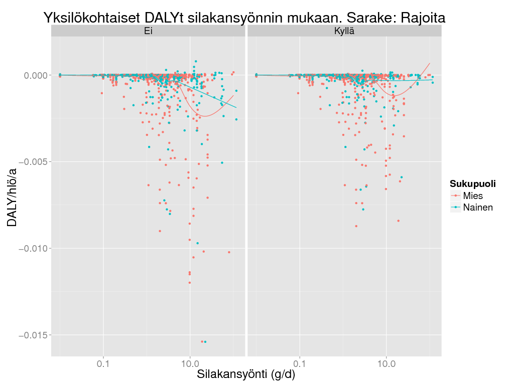
> sil <- unique(suomenna(daly)[c("Iter", "Ikäryhmä", "Sukupuoli", "Rajoita", "Silakkamäärä")])
> sil <- merge(sil, suomenna(dalyi))
> ggplot(subset(sil, as.integer(as.character(Iter)) <= 1000) , aes(x = Silakkamäärä, y = Result, colour = Sukupuoli)) + geom_point() + geom_smooth() +
+ scale_x_log10() + facet_grid(. ~ Rajoita) + theme_gray(base_size = BS) +
+ labs(
+ title = "Yksilökohtaiset DALYt silakansyönnin mukaan. Sarake: Rajoita",
+ x = "Silakansyönti (g/d)",
+ y = "DALY/hlö/a"
+ )
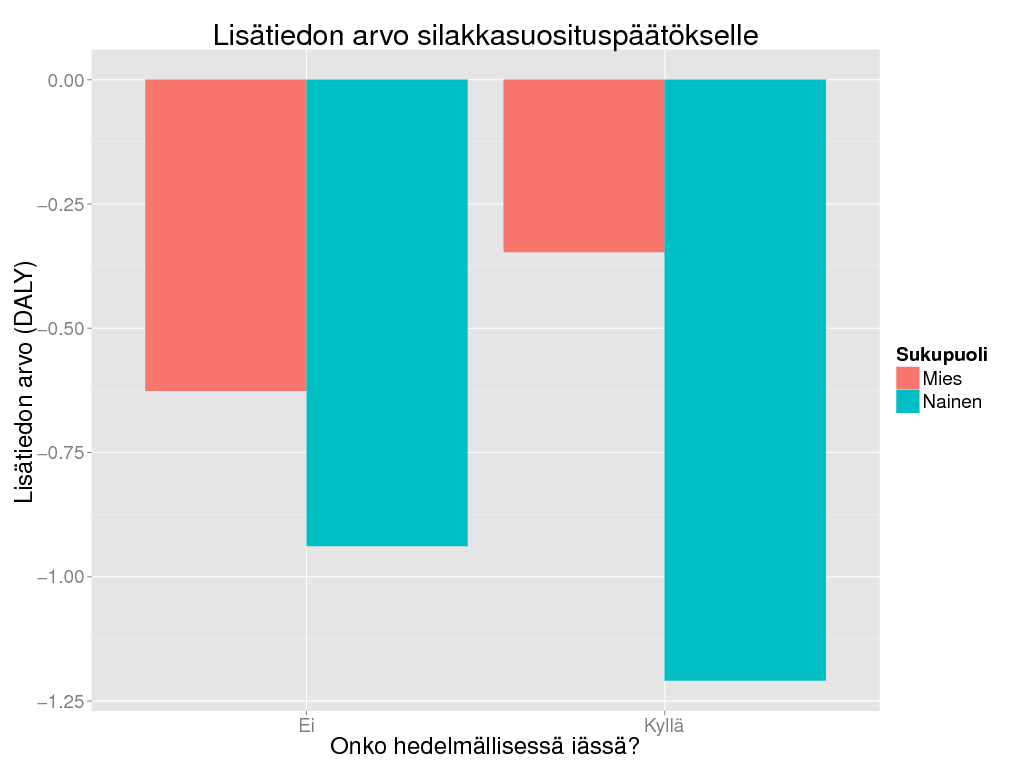
> ############################# YKSILÖTASON VOI
> dalyvoi <- oapply(daly, cols = "Trait", FUN = "sum")
> dalyvoi <- VOI(dalyvoi, dec = "Rajoita")
> dalyvoi <- oapply(dalyvoi * pophed, cols = "Age", FUN = "sum") # Population per sex
> ggplot(suomenna(dalyvoi), aes(x = Hedelm, weight = Result, fill = Sukupuoli)) +
+ geom_bar(position = "dodge") + theme_gray(base_size = BS) + #theme(axis.text.x = element_text(angle = 90, hjust = 1)) +
+ labs(
+ title = "Lisätiedon arvo silakkasuosituspäätökselle",
+ y = "Lisätiedon arvo (DALY)",
+ x = "Onko hedelmällisessä iässä?"
+ )
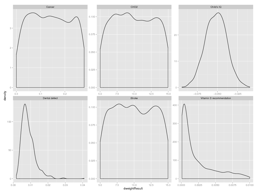
> ######### Plot disability weights
> dweight <- EvalOutput(dweight)
> ggplot(subset(dweight@output, Trait %in% c(
+ "Cancer",
+ "CHD2",
+ "Stroke",
+ "Child's IQ",
+ "Dental defect",
+ "Vitamin D recommendation"
+ )), aes(x = dweightResult))+geom_density()+facet_wrap(~ Trait, scale = "free")
> ######## Fill in the missing Age * Iter combinations by inputing
> # This converts Age into marginal.
> # This must be done, otherwise aggragation by oapply results in too small values.
> dalypinp <- daly * pophed
> N <- length(unique(dalypinp@output$Iter))
> rows <- unlist(tapply(1:nrow(dalypinp@output),
+ dalypinp@output[c("Trait", "Sukupuoli", "Hedelm", "Rajoita", "Age")],
+ FUN = function(x) sample(x, N, replace = TRUE)
+ ))
> dalypinp@output <- dalypinp@output[rows , ]
> dalypinp@output$Iter <- 1:N # From now on the Iter does not match that of any other variable
> dalypinp@marginal[colnames(dalypinp@output) == "Age"] <- TRUE
> oprint(summary(oapply(dalypinp, cols = c("Age", "Hedelm", "Trait"), FUN = sum), fun = c("mean", "sd", "Q0.025", "Q0.975")), digits = 1)

> oprint(summary(oapply(dalypinp, cols = c("Age", "Hedelm", "Sukupuoli"), FUN = sum), fun = c("mean", "sd", "Q0.025", "Q0.975")), digits = 1)

> oprint(summary(oapply(dalypinp, cols = c("Age", "Trait"), FUN = sum), fun = c("mean", "sd", "Q0.025", "Q0.975")), digits = 1)

> oprint(summary(oapply(dalypinp, cols = c("Hedelm", "Trait"), FUN = sum), fun = c("mean", "sd", "Q0.025", "Q0.975")), digits = 1)

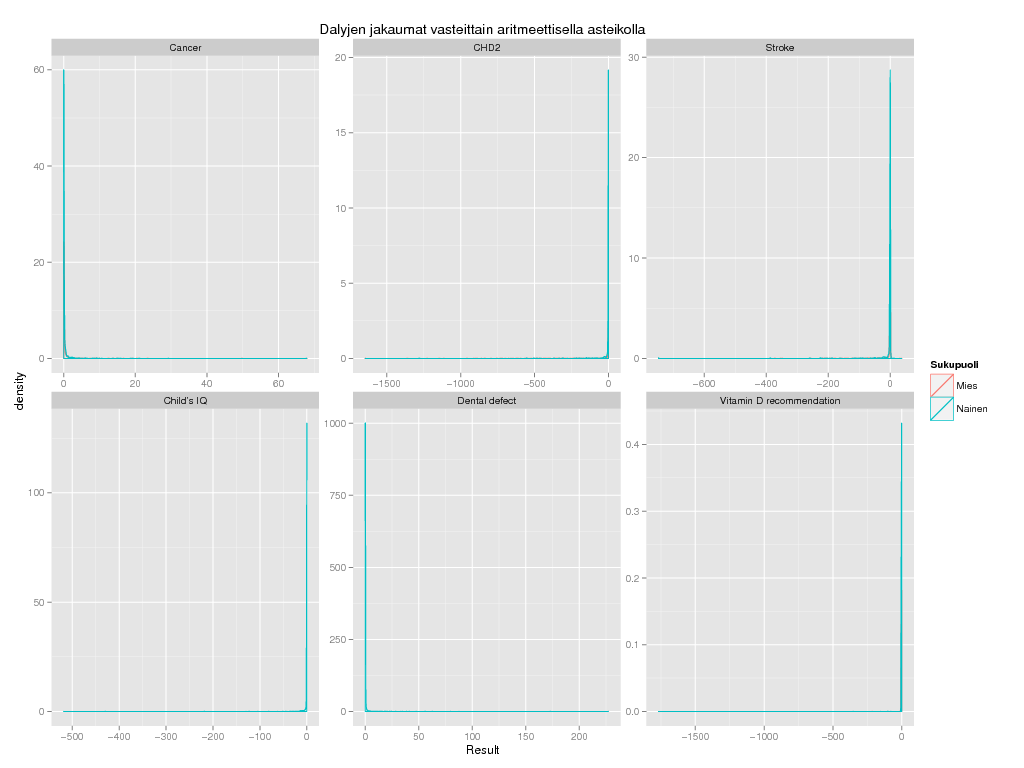
> ######## DALY distributions by trait
> ggplot(subset(dalypinp@output, !Trait %in% c("Child's IQ", "Dental defect") | Sukupuoli == "Nainen") ,
+ aes(x = Result, colour = Sukupuoli)) + geom_density() + facet_wrap(~ Trait , scale = "free") +
+ labs(title = "Dalyjen jakaumat vasteittain aritmeettisella asteikolla")
> ggplot(subset(dalypinp@output, !Trait %in% c("Child's IQ", "Dental defect") | Sukupuoli == "Nainen") ,
+ aes(x = abs(Result), colour = Rajoita)) + geom_density() + facet_wrap(~ Trait , scale = "free") +
+ scale_x_log10() + labs(title = "Absoluuttidalyt log-asteikolla")